Computational pipeline#
The following text is from Vennell et al. (2025).
At a high level, particle tracking code takes the Eulerian water velocity field from a hydrodynamic model and interpolates these velocities to provide velocities at particle locations, and then numerically integrates these to give particle trajectories. In addition, there are multiple other processes and computations that must be done at each time step. Such as the physical processes of dispersion, resuspension and tidal stranding, along with multiple bookkeeping processes. OceanTracker decomposes these processes into a series of components that fulfil specific roles, as part of the computational pipeline outlined in Figure 3. Figure 2 illustrates the data flow in OceanTracker from hydrodynamic model files to outputs, via its two main data structures: fields and particle properties. Fields store data from the hydrodynamic model, such as water velocity, salinity, wind stress, as well as custom fields which are calculated from other fields, such as friction velocity. Particle properties hold data for each particle, which could include their current locations, status or temperature. These data structures enable access to, and operations on, their data and are collectively “managed” by their respective manager roles.
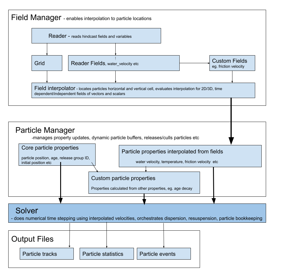
Figure 2: Outline of data flow through the two main data structures, fields and particle properties, from hydrodynamic model files to output. Each have “managers” to orchestrate operations on the variants of each data structure, to deliver particle properties to the solver. The steps carried out by the solver are given in Fig. 3.#
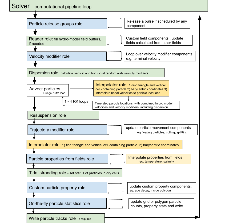
Figure 3: Flow chart of time stepping to advect particles within the solver component in Fig. 2. The figure illustrates the order in which components are updated within their roles in the computational pipeline . Green are “core roles” which only containing one component, blue roles may contain one or more components which are looped through. For large runs, the most computational expensive steps are 1.) finding the cell containing each particle and 2.) evaluating the field interpolation. These steps are coloured yellow#
The computational pipeline is constructed from components assigned to specific roles within the pipeline which implement required tasks at each time step (see Figure 3). From a user’s perspective, the adaptability of OceanTracker comes from the ability to customise which components are added to each role to create a computational pipeline for their needs. For example, a gridded 2D statistic added to the ‘particle statistics’ role to create heatmaps of particle locations on-the-fly. These components are constructed as Python classes, which are dynamically added to the computational pipeline during setup. Time stepping within the computational pipeline proceeds by calling the “update” method of each component within each role. Some roles, such as dispersion and re-suspension, allow only one class to be added, while others allow multiple classes to be added to that role. For example, multiple trajectory modifiers can be combined to give the required particle behaviour.
Building a Computational Pipeline#
The computational pipeline in OceanTracker can be fully configured using parameters provided in either a JSON or YAML text file or a Python dictionary, eliminating the need for direct coding (see Figure 4b, c). For more complex simulations, parameters can be specified programmatically using a helper wrapper. This wrapper provides two key methods: settings and add_class, which enable users to construct a parameter dictionary using keyword arguments (see Figure 4a). The resulting parameter dictionary follows the same structure as the JSON text file format shown in Figure 4c and is passed to OceanTracker for execution.
Users can configure top-level settings, such as the particle tracking time step and output directories, as well as component-specific settings. This trajectory calculation process constitutes a series of roles performed by a collection of components. Each component’s configuration typically includes the name of the Python class assigned to a particular role. Most component settings have default values defined within their respective Python classes, but some class settings must be explicitly provided by the user. During setup, all user-defined settings are automatically validated for type correctness and appropriate value ranges. To run OceanTracker a user must add at least a reader class and one release group class. In addition, provide settings giving the folder where output is to be written and the base used to both name the output folder for the run and the start of the output file names, as done in Figure 4.
Computational Steps#
Time stepping in OceanTracker integrates particle velocity to compute trajectories. Within the computational pipeline, time stepping is divided into a series of roles, each performed by one or more components (see Figure 3). The update of each component is automated within the time stepping of the computational pipeline, with updates grouped by role. The order in which the roles are updated reflects their temporal dependence on the data from other roles. For example, custom particle properties may be calculated from field particle properties and are therefore updated after the interpolated field properties.
The solver class implements the time stepping by managing the classes within the computational pipeline and the associated bookkeeping functions.
The first step in the computational pipeline involves looping over the release groups and releasing a single pulse of particles if scheduled for the current time step, and then finding each newly released particle’s current horizontal and vertical cell. The solver then checks if the reader field time buffers contain the required time steps; if not, the reader fills the buffers and any custom fields are calculated from the newly read time steps. Next, any additional particle velocities are added together to give a total of “velocity modifiers” (e.g. a fall velocity), to this a random walk dispersion is added as an equivalent velocity. Particles are then advected by RK integration based on the sum of the water velocity and the total of the velocity modifiers. At each sub-step, their current horizontal and vertical cells and barycentric coordinates are updated, so that each particle’s velocity can be interpolated to their locations. By default, fourth order RK time integration is used, although first and second order RK are also available.
Once particles are at their new locations, additional changes to particle status or positions due to resuspension or specified trajectory modifiers are made. These modifiers add any additional particles movements or changes to their status, e.g. settling in a polygon or culling. To enable interpolation after these movements, particle horizontal and vertical cells and Barycentric coordinates are updated. Then, all field-derived particle properties are looped over and updated by interpolation. Subsequent steps include updating any custom particle properties, calculating any particle statistics that have been added to the computational pipeline, and then writing out time series of particle trajectories and particle properties if this has been requested.
Mechanisms Enabling Computational Pipeline Adaptability#
OceanTracker’s computational pipeline flexibility is implemented through several key mechanisms:
Dynamic importing: Components for all roles are dynamically imported at runtime, allowing users to build custom computational pipelines. To specify a component, users provide a “class name” setting, which follows standard Python class referencing conventions. Core roles have default class names, and all built-in OceanTracker classes can be imported using a shortened version of their full names. Users can also import customised variants of Python classes into any of the roles in the computational pipeline, enabling them to modify core functionality or add optional functionality (e.g. dispersion models, trajectory modifiers or on-the-fly statistics).
Inheritance: New component variants can be created by inheriting from an existing class. Users can modify computations by overwriting specific methods, such as the “update” method, while retaining inherited configuration settings and the infrastructure that manages bookkeeping operations. This approach allows for incremental modifications—settings from a parent class are automatically inherited but can be redefined, removed, or extended. For example, the polygon particle release class inherits most of its functionality from the point release parent class.
Internal naming: To simplify code interaction, OceanTracker provides standardised internal names for instances of the field and particle property components. Additionally, both reader-defined fields and custom user-defined fields automatically generate particle properties of the same name, which are interpolated at each time step and can be accessed directly in the code. Users can also assign names to optional components for easier reference within their scripts. For example, essential fields like “water velocity” and “water depth” are mapped to corresponding variables in the hydrodynamic model files by the reader. Vector fields may require mapping multiple file variables to a single internal name.
Data Structures#
OceanTracker’s two main data structures are fields and particle properties (see Figure 2). This section outlines these data roles, while the next section describes their management.
Field Role#
The spatial fields stored within the hydrodynamic model’s files are the foundation of offline particle tracking. These are stored and accessed using the “field” data structure (see Figure 2). The water velocity field is a crucial spatial field for particle tracking, but there may be many other relevant fields, such as water depth, tide or wind-stress. OceanTracker automatically detects whether fields are 2D or 3D, time-dependent or independent, scalar or vector, and manages them appropriately. There are also grid variables associated with the fields, including nodal locations, triangulation and cell adjacency.
Fields are read from hydrodynamic model files as described in the Reader Role section. Users can also integrate custom fields into the computational pipeline by deriving new values from existing fields. For example, a friction velocity field can be computed from the 3D velocity field near the seabed to determine whether a particle can be re-suspended by the flow.
Particle Property Role#
There are three types of particle properties which store the values for each particle and enable high level operations on these values as shown in Figure 2b. These properties can have different types depending on how they are updated at each time step, and may be integer, scalars or vectors.
Field particle properties store field values at each particle location and are updated by interpolating a field data structure, e.g. water velocity.
Core particle properties are updated within the core code, i.e. outside of their class update method. Examples include particle location and bookkeeping particle properties, such as particleID, release groupID, or particle status, e.g. whether computationally alive, on the sea bed, stranded by the tide etc.
Custom particle properties store values calculated from other particle properties. For example, the “inside-polygons” class uses the location particle property to determine whether any user-given polygon contains each particle. These are updated by calling their class’s update method.
Some examples of currently available custom particle properties are:
Age decay which models an exponentially decaying particle load, such as bacteria, based on the core “age” particle property
Inside polygon records the polygons, from a given set, containing a particle. This information is used to compute polygon connectivity statistics or to determine events such as larval settlement when a particle drifts over a reef.
Total water depth which represents the sum of tidal elevation and water depth. This property is useful for particles whose behaviour differs in different water depths, such as larvae that only settle in shallow water, even if a cell is not completely dry.
Manager Roles#
Instances of field and particle properties store, update, and manage access to individual data values. Higher level operations on all the individual instances are orchestrated by “managers” which automate key processes (see Figure 2).
Fields Group Manager Role#
This orchestrates the setup, reading, updating and interpolation of fields, along with setting up the required grid variables, such as nodal locations, triangulation and the adjacency matrix. It also manages the process of finding each particle’s current horizontal and vertical cell, and updates the status of dry cells. By default, the fields group manager automatically adds a particle property with the same internal name as the field to the computational pipeline, to be interpolated at each time step. When nesting small fine-scale grids within a larger outer grid, a special fields group manager creates a Fields group manager for each grid. It associates each particle with the appropriate grid, so that their water velocity and other particle properties can be interpolated from the fields of that grid. At each time step, any particles crossing the open boundaries of the inner grid are associated with the outer grid. Conversely, any particles on the outer grid that move inside an inner grid are then associated with that grid.
Particle Group Manager Role#
This manages the release of particles and the updating of all three types of particle properties. It also manages the dynamic memory buffers which hold the individual particle property values, expanding them as needed when particle numbers grow and culling computationally dead particles that are no longer of interest. Additionally, if required, this manager handles the writing of time series of particle trajectories and properties.
Reader Role#
The primary function of the reader is to convert hydrodynamic model file variables into standardised internal formats, which may be stored in different files. The reader builds a catalogue of all file variables and which files contain them. It then maps the file variables to standard internal variable names. Field variables are categorised as time varying, vector or 3D. For vector variables, e.g. water velocity, several file variable names can be mapped to a single internal vector variable, allowing vector fields to be treated as a single variable within computations.
To ensure files for time-varying variables are read in the correct order, files are sorted into time order, using the hindcast’s time variable. Thus OceanTracker is not reliant on a file naming convention to determine file order. Each variable has its own list of files, which enables the reader to seamlessly accommodate hydrodynamic models where variables are split between files, as is the case for SCHISM version 5 output files and NEMO/GLORYS output files.
The reader loads fields into memory buffers as they are needed. For time-dependent variables it reads multiple time steps into buffers, if the next time step is not already in the buffer. By default, the buffer maintains 24 hydrodynamic model time steps in memory. This default number of steps balances enhancing speed by reading in multiple time steps at the same time, while only requiring 100s of megabytes of computer RAM for each buffered hindcast variable.
If needed, the reader converts the non-nodal values to values at the nodes of the triangles through interpolation. Readers and interpolators based on a hydrodynamic model’s native grid, that do not need to do this conversion, could be developed in the future. To facilitate automation, the reader stores all fields in 4D arrays with dimensions corresponding to time, node, z-depth and vector components.
For the unstructured SCHISM and DELFT3D-FM grids, which can have a mixture of triangular and quad cells, quad cells are divided into triangles. This division simply took the first 3 nodes of a quad cell as one triangle, then created a new triangle from the third, fourth and first nodes. Modifying the ‘triangulation’ of the hydrodynamic model grid by splitting quad cells is only done once at the start of the run and has no impact on the time spent reading the hindcast. It also adds little to the memory used, as the underlying field values are still stored as nodal values. By increasing the number of cells to search, quad cell splitting may slightly increase the time taken to locate the cell containing each particle. However, it simplifies the code by only requiring one type of cell to search.
Interpolator Role#
The interpolator serves as the link between the hydrodynamic model’s fields held by the reader and the corresponding particle properties. The interpolator has two functions: 1) determining each particle’s current horizontal and vertical cell, 2) interpolating field values at the triangles’ vertices to each particle’s location, which are then stored as particle properties. In the horizontal, OceanTracker currently uses linear interpolation in unstructured triangular grids from nodal values, utilizing a particle’s Barycentric coordinates within their current triangle, along with linear interpolation between hydrodynamic model time steps.
Vertical interpolation to each particle’s position is also linear between the layers of the hydrodynamic model and between time steps. The one exception to linear vertical interpolation is the water velocity within the seabed layer. Here, vertical interpolation is based on a logarithmic layer, ensuring that particles near the seabed experience more realistic horizontal velocities.
The interpolator supports linear interpolation for several vertical grids: Sigma grid (ROMS, DELFT-3D FM) and fixed z levels (DELFT-3D FM, NEMO/GLORYS), which apply the same vertical grid at all locations. It also supports grids with spatially varying layer thicknesses (SCHISM, FVCOM). This includes SCHISM’s LSC vertical grid, where the number of vertical layers also varies spatially.
Particle Release Groups Role#
A “particle release group” introduces new particles into the computational pipeline. Each release group generates new particles at specified locations, which are released at designated times, in specified pulse sizes. Multiple release groups can be added, each with their specific release locations and release schedules. Release groups can be:
Point release spawns particles from a set of specified locations and depths, such as the two crosses in the middle of the plots in Figure 1. A radius release class releases particles randomly within a circular area around each point.
Polygon release: Particles are spawned at random locations within a user-defined 2D polygon, e.g. mid-right of the upper plots in Figure 1.
Grid release: spawns particles from points of a regular grid, as on the upper left of the upper plots in Figure 1.
Particles will not be released on land, e.g. where a release polygon overlaps land as in Figure 1a. By default, particles are not released within cells that are currently dry due to the tide. For all types it is possible to restrict releases to be randomly distributed within a given vertical layer, or to locations with water depth within a given range.
Velocity Modifiers Role#
Additional bio-physical processes can be added to the water velocity experienced by each particle. These are incorporated into the computational pipeline as “velocity modifiers”, which are added to the water velocity for use in the time integration (Figure 3). An example of an in-built modifier is:
Terminal velocity: The modifier adds the terminal sinking or buoyant velocity to the ambient water velocity, either as a uniform value or a particle specific value drawn from a normal distribution.
Trajectory Modifiers Role#
“Trajectory modifiers” are bio-physical processes that alter the movement of particles at each time step or their status. Examples of in-built modifiers include:
Settlement: Allows particles to settle within user defined polygons, e.g. larvae to settle on reefs. The trajectory is modified by changing its status to “stationary”.
Floating: Sets each particle’s vertical position to that of the free-surface height at its current location.
Culling: Sets the status of a random fraction of particles for a given status (e.g. on the bottom) to be dead, allowing them to be removed from subsequent computations and particle statistics.
Splitting: Splits particles in two to simulate reproduction, at a set rate or probability. This can rapidly generate very large numbers of particles, which may need to be contained by a culling mechanism.
On-the-fly Particle Statistics Roles#
OceanTracker employs an on-the-fly particle counting approach to produce particle statistics during the computational run. This produces a data output volume that is independent of the total number of released particles. Currently available spatial particle statistics are:
Gridded: Count particles inside the cells of a regular grid at user-specified time intervals. These are commonly used to generate heat maps (see Figure 1).
Polygon: Compute the physical connectivity matrix between each release group and user-defined polygonal regions.
Both gridded and polygon-based statistics can be recorded using two approaches:
Time Series: Counts particles at specified time intervals, producing time-based heat maps or connectivity data.
Age Bin Series: Categorises particles into age bins within each spatial region, enabling the generation of age-based heat maps or connectivity matrices.
Users can filter which particles are counted, such as restricting statistics to particles within a specific vertical range or to particles resting on the seabed. Multiple on-the-fly statistics components can be combined, allowing, for example, separate particle counts for different depth layers.
Beyond counting particles, average values of particle properties can also be computed within the spatial bins. For instance, users can track average water temperature of particles within a given grid cell or polygon.
Integrated Models#
Users may need to combine multiple roles to create higher level functionality. OceanTracker supports this aggregation of roles into a single component, facilitating wider use of that functionality and collaboration. These integrated models only require the parameters essential for executing their higher-level function; the model manages the intricacies of assigning classes to appropriate roles to complete the overall function. Currently, there is one integrated model:
On-the-fly Lagrangian Coherent Structures: These structures identify regions of convergence or divergence within a fluid flow over time. OceanTracker calculates time series of Finite-Time Lyapunov Exponents (FTLE), which can be used to derive characteristics of Lagrangian Coherent Structures. The FTLE calculation uses the largest Eigenvalue of the strain tensor after specified lag times. This process involves releasing particles on a regular grid and calculating the distances between adjacent released particles. The user only needs to designate one or more grid locations and the required time lags. The integrated model sets up new regular grid releases at regular time intervals and calculates the FTLE on-the-fly for each grid and lag, eliminating the need to record and post process large volumes of particle trajectories.