Minimal example#
[This notebook is distributed as part of OceanTracker’s source code oceantracker/tutorials_how_to/]
Running a simulation generally follows three steps:
Define model parameters
Pass these parameters to OceanTracker and running the model
Visualize the results
This example uses OceanTracker’s “helper functions” - a set of python methods - to configure and run OceanTracker. You can also run OceanTracker from the command line uns using json or yaml input files. See tutorial E: using parameter dictionaries for more info on that.
# Notes for debugging if the scripts below fail:
# * These scripts assume that you already installed oceantracker. If you didn't, take a look at https://oceantracker.github.io/oceantracker/_build/html/info/installing.html
# * Paths in this directory are relative to the location of the ipython notebook.
#   I.e. On Linux or Mac, running a cell with "!ls" should return a list containing the notebook you are running.

# Checks if the hindcast data is available and download them if not
from oceantracker.util.download_data import download_hindcast_data_for_tutorials
download_hindcast_data_for_tutorials()
Hindcast data found locally at ./demo_hindcast
import os  # used here exclusively to make platform (win/mac/linux) dependent paths
from oceantracker.main import OceanTracker
prelim: Starting package set up
# minimal_example.py using class helper method
# ------------------------------------------------

# create an oceantracker instance that we can then configure step by step
ot = OceanTracker()

# ot.settings method use to set basic settings
ot.settings(
    run_output_dir=os.path.join("output", "minimal_example"),
    time_step=120,  #  2 min time step as seconds
)

# the different functionality is contained in "classes"
# here we add the 'reader' to read the hydrodynamical hindcasts
ot.add_class(
    "reader",
    # folder to search for hindcast files, sub-dirs will, by default, also be searched
    input_dir="./demo_hindcast/schsim3D",
    # hindcast file mask - only read files that follow this pattern
    file_mask="demo_hindcast_schisim3D*.nc",
)

# next we add "release groups" to define where, when and how particles are released
# you can multiple release groups for different kinds of releases (point or polygon)
# or to keep them apart in the results
ot.add_class(
    "release_groups",
    points=[
        [1595000, 5482600],  # [x,y] pairs of release locations
        [1599000, 5486200],
    ],  # must be an N by 2 or 3 or list, convertible to a numpy array
    release_interval=3600,  # seconds between releasing particles
    pulse_size=10,  # number of particles released each release_interval
)

# we can already run this minimal setup
case_info_file_name = ot.run()
helper: ----------------------------------------------------------------------
helper: Starting OceanTracker helper class,  version 0.5.2.55
helper:      Python version: 3.11.14 | packaged by conda-forge | (main, Oct 22 2025, 22:46:25) [GCC 14.3.0]
helper: ----------------------------------------------------------------------
helper: OceanTracker version 0.5.2.55  starting setup helper "main.py":
helper: Started
helper: Output is in dir "/home/ls/projects/oceantracker_dev/oceantracker/tutorials_how_to/output/minimal_example"
helper:     hint: see for copies of screen output and user supplied parameters, plus all other output
helper:     >>> Note: to help with debugging, parameters as given by user  are in "raw_user_params.json"
helper: ----------------------------------------------------------------------
helper: Numba setup: applied settings, max threads = 32, physical cores = 32
helper:     hint:  cache code = False, fastmath= False
helper: ----------------------------------------------------------------------
loading oceantracker read files
helper:       - Built OceanTracker package tree,      0.983 sec
helper:       - Built OceanTracker sort name map,     0.000 sec
helper:   - Done package set up to setup ClassImporter,       0.983 sec
setup: ----------------------------------------------------------------------
setup:  OceanTracker version 0.5.2.55
setup:     Starting user param. runner at 2026-01-21T17:42:26.986541
setup: ----------------------------------------------------------------------
setup:   - Start  field group manager and readers setup
setup:   - Found input dir "./demo_hindcast/schsim3D"
setup:   - Detected reader class_name = "oceantracker.reader.SCHISM_reader.SCHISMreader"
setup:   - Starting grid setup
setup:     - built node to triangles map,     0.887 sec
setup:     - built triangle adjacency matrix,         0.191 sec
setup:     - found boundary triangles,        0.000 sec
setup:     - built domain and island outlines,        1.085 sec
setup:     - calculated triangle areas,       0.000 sec
setup:   - Finished grid setup
setup: --- Hindcast info ----------------------------------------------------
setup:     Hydro-model is "3D", type "SCHISMreader"
setup:         hint: Files found in dir and sub-dirs of "./demo_hindcast/schsim3D"
setup:         Geographic coords = "False"
setup:         Hindcast start: 2017-01-01T00:30:00  end:  2017-01-01T23:30:00
setup:           time step = 0 days 1 hrs 0 min 0 sec, number of time steps= 24
setup:           grid bounding box = [1589789.000 5479437.000] to [1603398.000 5501640.000]
setup:           has:  A_Z profile=True,  bottom stress=False, regrid to sigma=True
setup:           vertical grid type = "LSC", using vertical grid  "Sigma"
setup: ----------------------------------------------------------------------
setup:   - Built barycentric-transform matrix,        0.340 sec
setup:   - Loading reader fields ['water_depth', 'tide', 'water_velocity']
setup:   - Finished field group manager and readers setup,    4.769 sec
setup: ----------------------------------------------------------------------
setup:   - Added 1 release group(s) and found run start and end times,        1.878 sec
setup:   - Starting initial setup of all classes
setup:     - Done initial setup of all classes,       0.004 sec
setup: ----------------------------------------------------------------------
setup:   - Starting "minimal_example",  duration: 0 days 23 hrs 0 min 0 sec
setup:       From 2017-01-01T00:30:00 to  2017-01-01T23:30:00
setup:       Time step 120.0 sec
setup:         using: A_Z_profile = False, bottom_stress = False
setup: ----------------------------------------------------------------------
setup:   -  Reading 24 time steps,  for hindcast time steps 00:23 into ring buffer offsets 000:023 ,  for run "None"
setup:       -  read  24 time steps in  1.2 sec, from ./demo_hindcast/schsim3D
setup:   - Starting time stepping: 2017-01-01T00:30:00 to 2017-01-01T23:30:00
setup:     duration  0 days 23 hrs 0 min 0 sec, time step=  0 days 0 hrs 2 min 0 sec
S:   - Opened tracks output and done written first time step in: "tracks_compact_000.nc",     0.129 sec
S: 0000: 00%:H0000b00-01 Day +00 00:00 2017-01-01 00:30:00: Rel:20   : Active:20     Move:20     Bottom:0     Strand:0      Dead:0     Out:   0 Buffer: 4%  step time = 9516.9 ms
S: 0030: 04%:H0001b01-02 Day +00 01:00 2017-01-01 01:30:00: Rel:40   : Active:40     Move:40     Bottom:0     Strand:0      Dead:0     Out:   0 Buffer: 8%  step time =  5.2 ms
S: 0060: 09%:H0002b02-03 Day +00 02:00 2017-01-01 02:30:00: Rel:60   : Active:60     Move:60     Bottom:0     Strand:0      Dead:0     Out:   0 Buffer:12%  step time =  5.2 ms
S: 0090: 13%:H0003b03-04 Day +00 03:00 2017-01-01 03:30:00: Rel:70   : Active:70     Move:60     Bottom:0     Strand:10     Dead:0     Out:   0 Buffer:14%  step time =  7.6 ms
S: 0120: 17%:H0004b04-05 Day +00 04:00 2017-01-01 04:30:00: Rel:80   : Active:80     Move:70     Bottom:0     Strand:10     Dead:0     Out:   0 Buffer:16%  step time =  7.6 ms
S: 0150: 22%:H0005b05-06 Day +00 05:00 2017-01-01 05:30:00: Rel:90   : Active:90     Move:80     Bottom:0     Strand:10     Dead:0     Out:   0 Buffer:18%  step time =  7.4 ms
S: 0180: 26%:H0006b06-07 Day +00 06:00 2017-01-01 06:30:00: Rel:100  : Active:100    Move:90     Bottom:0     Strand:10     Dead:0     Out:   0 Buffer:20%  step time =  6.7 ms
S: 0210: 30%:H0007b07-08 Day +00 07:00 2017-01-01 07:30:00: Rel:110  : Active:110    Move:100    Bottom:0     Strand:10     Dead:0     Out:   0 Buffer:22%  step time =  7.3 ms
S: 0240: 35%:H0008b08-09 Day +00 08:00 2017-01-01 08:30:00: Rel:120  : Active:120    Move:110    Bottom:0     Strand:10     Dead:0     Out:   0 Buffer:25%  step time =  5.5 ms
S: 0270: 39%:H0009b09-10 Day +00 09:00 2017-01-01 09:30:00: Rel:140  : Active:140    Move:140    Bottom:0     Strand:0      Dead:0     Out:   0 Buffer:29%  step time = 10.6 ms
S: 0300: 43%:H0010b10-11 Day +00 10:00 2017-01-01 10:30:00: Rel:160  : Active:160    Move:160    Bottom:0     Strand:0      Dead:0     Out:   0 Buffer:33%  step time =  7.4 ms
S: 0330: 48%:H0011b11-12 Day +00 11:00 2017-01-01 11:30:00: Rel:180  : Active:180    Move:180    Bottom:0     Strand:0      Dead:0     Out:   0 Buffer:37%  step time =  7.3 ms
S: 0360: 52%:H0012b12-13 Day +00 12:00 2017-01-01 12:30:00: Rel:200  : Active:200    Move:200    Bottom:0     Strand:0      Dead:0     Out:   0 Buffer:41%  step time = 14.1 ms
S: 0390: 57%:H0013b13-14 Day +00 13:00 2017-01-01 13:30:00: Rel:220  : Active:220    Move:205    Bottom:0     Strand:15     Dead:0     Out:   0 Buffer:45%  step time =  8.0 ms
S: 0420: 61%:H0014b14-15 Day +00 14:00 2017-01-01 14:30:00: Rel:240  : Active:240    Move:221    Bottom:0     Strand:19     Dead:0     Out:   0 Buffer:50%  step time =  7.9 ms
S: 0450: 65%:H0015b15-16 Day +00 15:00 2017-01-01 15:30:00: Rel:250  : Active:250    Move:192    Bottom:0     Strand:58     Dead:0     Out:   0 Buffer:52%  step time =  8.5 ms
S: 0480: 70%:H0016b16-17 Day +00 16:00 2017-01-01 16:30:00: Rel:260  : Active:260    Move:193    Bottom:0     Strand:67     Dead:0     Out:   0 Buffer:54%  step time =  9.1 ms
S: 0510: 74%:H0017b17-18 Day +00 17:00 2017-01-01 17:30:00: Rel:270  : Active:270    Move:195    Bottom:0     Strand:75     Dead:0     Out:   0 Buffer:56%  step time =  7.8 ms
S: 0540: 78%:H0018b18-19 Day +00 18:00 2017-01-01 18:30:00: Rel:280  : Active:280    Move:205    Bottom:0     Strand:75     Dead:0     Out:   0 Buffer:58%  step time =  8.8 ms
S: 0570: 83%:H0019b19-20 Day +00 19:00 2017-01-01 19:30:00: Rel:290  : Active:290    Move:217    Bottom:0     Strand:73     Dead:0     Out:   0 Buffer:60%  step time = 10.2 ms
S: 0600: 87%:H0020b20-21 Day +00 20:00 2017-01-01 20:30:00: Rel:300  : Active:300    Move:236    Bottom:0     Strand:64     Dead:0     Out:   0 Buffer:62%  step time =  7.5 ms
S: 0630: 91%:H0021b21-22 Day +00 21:00 2017-01-01 21:30:00: Rel:320  : Active:320    Move:301    Bottom:0     Strand:19     Dead:0     Out:   0 Buffer:66%  step time = 10.3 ms
S: 0660: 96%:H0022b22-23 Day +00 22:00 2017-01-01 22:30:00: Rel:340  : Active:340    Move:325    Bottom:0     Strand:15     Dead:0     Out:   0 Buffer:70%  step time =  8.3 ms
S: 0690: 100%:H0022b22-23 Day +00 23:00 2017-01-01 23:30:00: Rel:360  : Active:360    Move:360    Bottom:0     Strand:0      Dead:0     Out:   0 Buffer:75%  step time =  8.4 ms
S: --- Closing all classes ----------------------------------------------
S: Converting compact track files to rectangular format (to disable set reader param convert=False)
S:     hint: reading from dir /home/ls/projects/oceantracker_dev/oceantracker/tutorials_how_to/output/minimal_example
S:     - Finished "tracks_rectangular_000.nc",        0.091 sec
S:     - Conversion complete,         0.091 sec
S: Removing compact track files output after conversion
end: ----------------------------------------------------------------------
end: Finished "minimal_example"
end:     Timings: total =  29.0 sec
end:         Setup                          1.20 s    4.1%
end:         Find initial horizontal cell   1.57 s    5.4%
end:         Reading hindcast               1.21 s    4.2%
end:         Find horizontal cell           2.49 s    8.6%
end:         Find vertical cell             1.53 s    5.3%
end:         Interpolate fields             1.47 s    5.1%
end:         Update custom particle prop.   0.00 s    0.0%
end:         Update statistics              0.00 s    0.0%
end:         Update event loggers           0.00 s    0.0%
end:         RK integration                 0.46 s    1.6%
end:         Releasing particles            0.05 s    0.2%
end:         Close down                     3.83 s   13.2%
end:         resuspension                   0.40 s    1.4%
end:         dispersion                     0.54 s    1.9%
end:         tracks_writer                  0.07 s    0.2%
end: ----------------------------------------------------------------------
end: Finished "minimal_example",  started: 2026-01-21 17:42:25.788022, ended: 2026-01-21 17:42:54.817729
end:       Computational time = 0:00:29.029719
end:       Max. memory used 111.27 GB
end: --- Issues    (check above,  any errors repeated below) --------------
end:     0 errors,    0 strong warnings,   0 warnings,   1 notes
end: --- Successful completion: output in "output/minimal_example" --------
/home/ls/projects/oceantracker_dev/oceantracker/tutorials_how_to/output/minimal_example/caseInfo.json
# case_info file name contains the path to "head" model output, located in the run_output_dir
# its a json file that contains e.g. model statistics and model output file names
# which is handy for post-processing
print(case_info_file_name)
/home/ls/projects/oceantracker_dev/oceantracker/tutorials_how_to/output/minimal_example/caseInfo.json
Read and plot output#
from oceantracker.read_output.python import load_output_files
from oceantracker.plot_output import plot_tracks
# oceantracker has some build in plotting tools that we frequently use to
# take a quick look at the model output

# first we need to read particle track data
tracks = load_output_files.load_track_data(case_info_file_name)
Merging rectangular track files
     Reading rectangular track file "tracks_rectangular_000.nc"
# the have a quick look at what variables are available you can call
_ = [print(item) for item in tracks.keys()]  # show what is in tracks dictionary holds
particles_written_per_time_step
time_step_range
time
num_part_released_so_far
x
x0
status
status_last_good
age
ID
IDrelease_group
user_release_groupID
IDpulse
hydro_model_gridID
time_released
water_depth
tide
dry_cell_index
grid
particle_status_flags
particle_release_groups
axis_lim
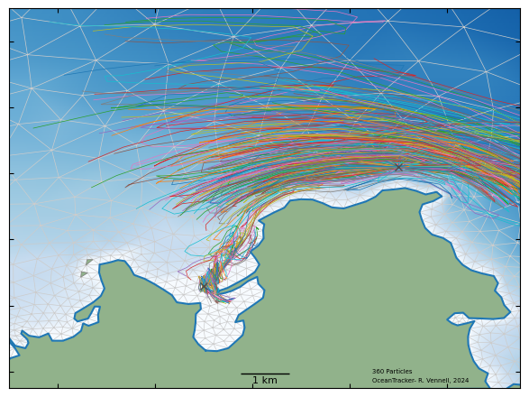
plot_tracks.plot_tracks(
    tracks, axis_lims=[1591000, 1601500, 5479500, 5491000], show_grid=True
)
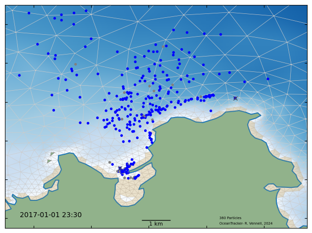
Add aminations#
In animation, sand colored area shows dry cells, blue particles are moving, green are stranded by the tide in dry cells, gray are on the sea bed, from which they resupend in this example.
By default particles are blocked from moving from a wet cell to a dry cell and will not be released if the release location lies within a dry cell.
from oceantracker.plot_output import plot_tracks
from IPython.display import HTML

# animate particles
anim = plot_tracks.animate_particles(
    tracks,
    axis_lims=[1591000, 1601500, 5479500, 5491000],
    interval=100, # milliseconds between frames
    show_dry_cells=True,
    show_grid=True,
    show=False, # we'll use the ipythons HTML function to show it
)

# this line only used in note books, in python scripts use show = True above
HTML(anim.to_html5_video())