Hydrodynamical models and helpful oceantracker utility functions

In the previous notebooks (A-E) we have focused on how oceantracker works, how to run it, some of its basic functionality, and how its output looks like. In these models we assumed that the underlying hydrodynamical model is already “understood” and we simply used some pre-defined release location, time-windows, etc. This is usually not the case when you design a new model. Finding available hydrodynamical models, deciding which to choose, and then to figure out all its detail is - assuming you are somewhat familiar with oceantracker already - is usually the most time consuming part of designing a model.

In this notebook we will take a quick look at an example workflow, and the available utilities that we offer that help in that process.

Hydrodynamical models are rather time consuming to produce, so there aren’t typically many to chose from. Sadly, the community is still fractured when it comes to making this model available. Many models are not cataloged, buried in some local government agency and only accessible upon request. If you don’t know what is available, the best thing is probably just to ask around, or look thru previous publications for the region of interest.

Visualizing the hydrodynamical model grid

Once you got access to a hydrodynamic model, you will need to figure out a few things first. 1. What is the coordinate system used? * If coordinates are provided in longitude and latitude they tend to be WGS84 (which is the basis of the GPS standard). Even if they are not, assuming WGS84 anyway usually gets you close enough to get something running until you manage to find some metadata or get in touch with someone who knows. * Many local i.e. coastal models however use specialized coordinate systems. These typically represent locations in meters relative to a particular map origin. To make sense of these you generally just need to know the map projection used. Figuring it out by yourself is rather time consuming. All common map projections are cataloged in the EPSG registry where they are given a unique label. E.g. WGS84 has the code “4326”. Once you know the coordinate system used, its seems to be always worthwhile to plot the model domain properly, to look at its grid, bathymetry, and crucial variables like current velocities

2. The next step is then to figure out the release locations for you particles. If you prefer, most of what is shown below can also be achieved with a GIS tool (e.g. QGIS) but if you are already familiar with python then doing it yourself in python - as we will illustrate - is probably easier.

# Notes for debugging if the scripts below fail:
# * These scripts assume that you already installed oceantracker. If you didn't take a look at https://oceantracker.github.io/oceantracker/_build/html/info/installing.html
# * Paths in this directory are relative to the location of the ipython notebook.
#   I.e. On Linux or Mac, running a cell with "!ls" should return a list containing the notebook you are running.

# Checks if the hindcast data is available and downloads them if not
from oceantracker.util.download_data import download_hindcast_data_for_tutorials
download_hindcast_data_for_tutorials()

Hindcast data found locally at ./demo_hindcast

# the previous notebooks used a small 3D SCHISM-based "toy"-model.
# Lets assume we just downloaded that hindcasts into ./demo_hindcast/ directory
# lets see whats there

import os
# to print the content of the directory:
os.listdir('demo_hindcast')

['make_demo_roms_hindcast.py',
 'ROMS',
 'make_demo_schism_hindcast.py',
 'schsim2D',
 'schsim3D']

# seems like schism3D is what we are looking for
# to print the content of the directory:
os.listdir(os.path.join('demo_hindcast','schsim3D'))

['demo_hindcast_schisim3D_00.nc']

# ".nc" abbreviation for netCDF,
# which is the current standard for sharing hydrodynamic data
# we can open that dataset using either netCDF4,
# or often a bit more conveniently using xarray
path_to_hindcast = os.path.join('demo_hindcast','schsim3D')
hindcast_files = [file for file in os.listdir(path_to_hindcast) if "nc" in file]

# lets use the first (and in our case only hindcast file)
# (xarray can also open several files at once using open_datasets)
first_file = hindcast_files[0]

import xarray as xr
ds = xr.open_dataset(os.path.join(path_to_hindcast,first_file))
# this will give you a quick overview
ds

<xarray.Dataset> Size: 4MB
Dimensions:                  (one: 1, nSCHISM_hgrid_face: 1106,
                              nMaxSCHISM_hgrid_face_nodes: 4,
                              nSCHISM_hgrid_node: 668, sigma: 38, time: 24,
                              nSCHISM_vgrid_layers: 8, two: 2)
Coordinates:
  * sigma                    (sigma) float32 152B 0.0 0.0 0.0 ... 0.0 0.0 0.0
  * time                     (time) datetime64[ns] 192B 2017-01-01T00:30:00 ....
Dimensions without coordinates: one, nSCHISM_hgrid_face,
                                nMaxSCHISM_hgrid_face_nodes,
                                nSCHISM_hgrid_node, nSCHISM_vgrid_layers, two
Data variables: (12/23)
    SCHISM_hgrid             (one) int32 4B ...
    SCHISM_hgrid_face_nodes  (nSCHISM_hgrid_face, nMaxSCHISM_hgrid_face_nodes) int32 18kB ...
    SCHISM_hgrid_node_x      (nSCHISM_hgrid_node) float32 3kB ...
    SCHISM_hgrid_node_y      (nSCHISM_hgrid_node) float32 3kB ...
    node_bottom_index        (nSCHISM_hgrid_node) int32 3kB ...
    depth                    (nSCHISM_hgrid_node) float32 3kB ...
    ...                       ...
    dahv                     (time, nSCHISM_hgrid_node, two) float32 128kB ...
    vertical_velocity        (time, nSCHISM_hgrid_node, nSCHISM_vgrid_layers) float32 513kB ...
    temp                     (time, nSCHISM_hgrid_node, nSCHISM_vgrid_layers) float32 513kB ...
    diffusivity              (time, nSCHISM_hgrid_node, nSCHISM_vgrid_layers) float32 513kB ...
    viscosity                (time, nSCHISM_hgrid_node, nSCHISM_vgrid_layers) float32 513kB ...
    hvel                     (time, nSCHISM_hgrid_node, nSCHISM_vgrid_layers, two) float32 1MB ...
Attributes:
    Conventions:   CF-1.0, UGRID-1.0
    title:         SCHISM Model output
    institution:   SCHISM Model output
    source:        SCHISM model output version v10
    references:    http://ccrm.vims.edu/schismweb/
    history:       created by combine_output11
    comment:       SCHISM Model output
    type:          SCHISM Model output
    VisIT_plugin:  https://schism.water.ca.gov/library/-/document_library/vie...

xarray.Dataset

• Dimensions:
  • one: 1
  • nSCHISM_hgrid_face: 1106
  • nMaxSCHISM_hgrid_face_nodes: 4
  • nSCHISM_hgrid_node: 668
  • sigma: 38
  • time: 24
  • nSCHISM_vgrid_layers: 8
  • two: 2
• Coordinates: (2)
  • sigma
    (sigma)
    float32
    0.0 0.0 0.0 0.0 ... 0.0 0.0 0.0 0.0

    long_name :

    S coordinates at whole levels

    units :

    1

    standard_name :

    ocean_s_coordinate

    positive :

    up

    h_s :

    0.0

    h_c :

    0.0

    theta_b :

    0.0

    theta_f :

    0.0

    formula_terms :

    s: sigma eta: elev depth: depth a: sigma_theta_f b: sigma_theta_b depth_c: sigma_h_c

    array([0., 0., 0., 0., 0., 0., 0., 0., 0., 0., 0., 0., 0., 0., 0., 0., 0., 0.,
           0., 0., 0., 0., 0., 0., 0., 0., 0., 0., 0., 0., 0., 0., 0., 0., 0., 0.,
           0., 0.], dtype=float32)

  • time
    (time)
    datetime64[ns]
    2017-01-01T00:30:00 ... 2017-01-...

    long_name :

    Time

    base_date :

    2017 1 1 0.00 0.00

    standard_name :

    time

    array(['2017-01-01T00:30:00.000000000', '2017-01-01T01:30:00.000000000',
           '2017-01-01T02:30:00.000000000', '2017-01-01T03:30:00.000000000',
           '2017-01-01T04:30:00.000000000', '2017-01-01T05:30:00.000000000',
           '2017-01-01T06:30:00.000000000', '2017-01-01T07:30:00.000000000',
           '2017-01-01T08:30:00.000000000', '2017-01-01T09:30:00.000000000',
           '2017-01-01T10:30:00.000000000', '2017-01-01T11:30:00.000000000',
           '2017-01-01T12:30:00.000000000', '2017-01-01T13:30:00.000000000',
           '2017-01-01T14:30:00.000000000', '2017-01-01T15:30:00.000000000',
           '2017-01-01T16:30:00.000000000', '2017-01-01T17:30:00.000000000',
           '2017-01-01T18:30:00.000000000', '2017-01-01T19:30:00.000000000',
           '2017-01-01T20:30:00.000000000', '2017-01-01T21:30:00.000000000',
           '2017-01-01T22:30:00.000000000', '2017-01-01T23:30:00.000000000'],
          dtype='datetime64[ns]')

• Data variables: (23)
  • SCHISM_hgrid
    (one)
    int32
    ...

    long_name :

    Topology data of 2d unstructured mesh

    topology_dimension :

    2

    cf_role :

    mesh_topology

    node_coordinates :

    SCHISM_hgrid_node_x SCHISM_hgrid_node_y

    face_node_connectivity :

    SCHISM_hgrid_face_nodes

    edge_coordinates :

    SCHISM_hgrid_edge_x SCHISM_hgrid_edge_y

    face_coordinates :

    SCHISM_hgrid_face_x SCHISM_hgrid_face_y

    edge_node_connectivity :

    SCHISM_hgrid_edge_nodes

    [1 values with dtype=int32]

  • SCHISM_hgrid_face_nodes
    (nSCHISM_hgrid_face, nMaxSCHISM_hgrid_face_nodes)
    int32
    ...

    long_name :

    Horizontal Element Table

    cf_role :

    face_node_connectivity

    start_index :

    1

    [4424 values with dtype=int32]

  • SCHISM_hgrid_node_x
    (nSCHISM_hgrid_node)
    float32
    ...

    long_name :

    node x-coordinate

    standard_name :

    projection_x_coordinate

    units :

    m

    mesh :

    SCHISM_hgrid

    [668 values with dtype=float32]

  • SCHISM_hgrid_node_y
    (nSCHISM_hgrid_node)
    float32
    ...

    long_name :

    node y-coordinate

    standard_name :

    projection_y_coordinate

    units :

    m

    mesh :

    SCHISM_hgrid

    [668 values with dtype=float32]

  • node_bottom_index
    (nSCHISM_hgrid_node)
    int32
    ...

    [668 values with dtype=int32]

  • depth
    (nSCHISM_hgrid_node)
    float32
    ...

    long_name :

    Bathymetry

    units :

    meters

    positive :

    down

    mesh :

    SCHISM_hgrid

    location :

    node

    [668 values with dtype=float32]

  • dry_value_flag
    (one)
    int32
    ...

    values :

    0: use last-wet value; 1: use junk

    [1 values with dtype=int32]

  • coordinate_system_flag
    (one)
    int32
    ...

    [1 values with dtype=int32]

  • minimum_depth
    (one)
    float32
    ...

    [1 values with dtype=float32]

  • sigma_h_c
    (one)
    float32
    ...

    long_name :

    ocean_s_coordinate h_c constant

    units :

    meters

    positive :

    down

    [1 values with dtype=float32]

  • sigma_theta_b
    (one)
    float32
    ...

    long_name :

    ocean_s_coordinate theta_b constant

    [1 values with dtype=float32]

  • sigma_theta_f
    (one)
    float32
    ...

    long_name :

    ocean_s_coordinate theta_f constant

    [1 values with dtype=float32]

  • sigma_maxdepth
    (one)
    float32
    ...

    long_name :

    ocean_s_coordinate maximum depth cutoff (mixed s over z boundary)

    units :

    meters

    positive :

    down

    [1 values with dtype=float32]

  • Cs
    (sigma)
    float32
    ...

    long_name :

    Function C(s) at whole levels

    positive :

    up

    [38 values with dtype=float32]

  • wetdry_elem
    (time, nSCHISM_hgrid_face)
    float32
    ...

    mesh :

    SCHISM_hgrid

    data_horizontal_center :

    elem

    data_vertical_center :

    full

    i23d :

    4

    ivs :

    1

    [26544 values with dtype=float32]

  • zcor
    (time, nSCHISM_hgrid_node, nSCHISM_vgrid_layers)
    float32
    ...

    mesh :

    SCHISM_hgrid

    data_horizontal_center :

    node

    data_vertical_center :

    full

    i23d :

    2

    ivs :

    1

    [128256 values with dtype=float32]

  • elev
    (time, nSCHISM_hgrid_node)
    float32
    ...

    mesh :

    SCHISM_hgrid

    data_horizontal_center :

    node

    data_vertical_center :

    full

    i23d :

    1

    ivs :

    1

    [16032 values with dtype=float32]

  • dahv
    (time, nSCHISM_hgrid_node, two)
    float32
    ...

    mesh :

    SCHISM_hgrid

    data_horizontal_center :

    node

    data_vertical_center :

    full

    i23d :

    1

    ivs :

    2

    [32064 values with dtype=float32]

  • vertical_velocity
    (time, nSCHISM_hgrid_node, nSCHISM_vgrid_layers)
    float32
    ...

    mesh :

    SCHISM_hgrid

    data_horizontal_center :

    node

    data_vertical_center :

    full

    i23d :

    2

    ivs :

    1

    [128256 values with dtype=float32]

  • temp
    (time, nSCHISM_hgrid_node, nSCHISM_vgrid_layers)
    float32
    ...

    mesh :

    SCHISM_hgrid

    data_horizontal_center :

    node

    data_vertical_center :

    full

    i23d :

    2

    ivs :

    1

    [128256 values with dtype=float32]

  • diffusivity
    (time, nSCHISM_hgrid_node, nSCHISM_vgrid_layers)
    float32
    ...

    mesh :

    SCHISM_hgrid

    data_horizontal_center :

    node

    data_vertical_center :

    full

    i23d :

    2

    ivs :

    1

    [128256 values with dtype=float32]

  • viscosity
    (time, nSCHISM_hgrid_node, nSCHISM_vgrid_layers)
    float32
    ...

    mesh :

    SCHISM_hgrid

    data_horizontal_center :

    node

    data_vertical_center :

    full

    i23d :

    2

    ivs :

    1

    [128256 values with dtype=float32]

  • hvel
    (time, nSCHISM_hgrid_node, nSCHISM_vgrid_layers, two)
    float32
    ...

    mesh :

    SCHISM_hgrid

    data_horizontal_center :

    node

    data_vertical_center :

    full

    i23d :

    2

    ivs :

    2

    [256512 values with dtype=float32]

• Attributes: (9)

  Conventions :

  CF-1.0, UGRID-1.0

  title :

  SCHISM Model output

  institution :

  SCHISM Model output

  source :

  SCHISM model output version v10

  references :

  http://ccrm.vims.edu/schismweb/

  history :

  created by combine_output11

  comment :

  SCHISM Model output

  type :

  SCHISM Model output

  VisIT_plugin :

  https://schism.water.ca.gov/library/-/document_library/view/3476283

# to just briefly introduce the netCDF standard:
# metadata -> ds.attrs (short for attributes)
# dimension -> ds.dims (gives you an idea of the "shape" of the data)
# data data -> ds['variables]

# be mindful tho that this data is only as good and well structured as somebody else felt like
# putting the effort in to follow standards and to fill out all the fields
# (i.e. sometimes these are a mess)

# for SCHISM models the variables that define the (horizontal) mesh are typically
x = ds['SCHISM_hgrid_node_x']
y = ds['SCHISM_hgrid_node_y']

# while most schism models use triangular grids, it also allows rectangles
# hence, by default "SCHISM_h(orizontal)grid_face_nodes"
# which defines which nodes are part a "face" of a prism or cube
# is (n,4) dimensional array
# schism also uses 1-based indexing
# hence, we slice for only the first three [:,:3]
# and we subtract one from all to values
# get to pythons zero based indexing
triangles = ds['SCHISM_hgrid_face_nodes'][:,:3] - 1

import matplotlib.pyplot as plt
plt.triplot(x, y, triangles)
plt.axis('equal') # to make sure we don't distort the projection

(np.float64(1589108.55),
 np.float64(1604078.45),
 np.float64(5478326.85),
 np.float64(5502750.15))

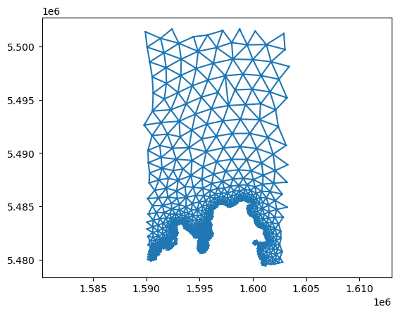
# taking a look at the axis labels,
# it looks like these aren't longitude/latitude values
# as these would be <360

# for this grid the NZTM projection was used which has the EPSG code of 2193
# to transform these to lon lat using WGS84 we can use the "pyproj" package

from pyproj import Transformer
transformer = Transformer.from_crs("EPSG:2193", "EPSG:4326", always_xy=True)
lon, lat = transformer.transform(x, y)

# we also offer a bunch of functionallity to deal with coord transformations
# from oceantracker.util.cord_transforms import convert_cords
# import numpy
# lon_lat = convert_cords(
#     np.stack([x, y], axis=1),
#     "EPSG:2193",
#     "EPSG:4326",
# )

plt.triplot(lon, lat, triangles, color='black', linewidth=0.5)
plt.xlabel('Longitude')
plt.ylabel('Latitude')
plt.axis('equal')

(np.float64(172.87104744825012),
 np.float64(173.048257317462),
 np.float64(-40.846102571740246),
 np.float64(-40.62605381761484))

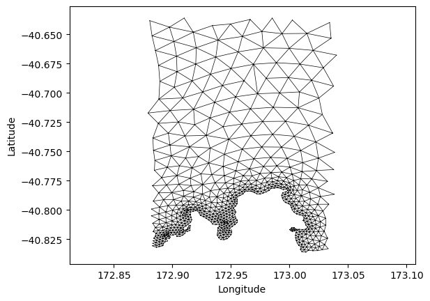
# great. that looks reasonable.
# we used some New Zealand based map projection and the lon lat values

# now, half the work is done.
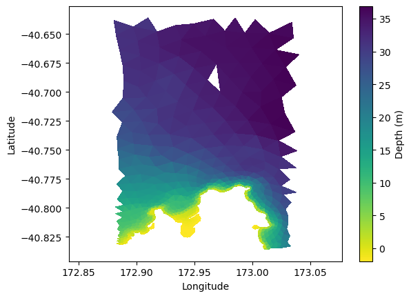
# we can plot some data to to check if the data set looks
# as we would expect it

Visualizing its data

plt.tripcolor(lon, lat, triangles, ds['depth'], cmap='viridis_r')
plt.xlabel('Longitude')
plt.ylabel('Latitude')
plt.axis('equal')
plt.colorbar(label='Depth (m)')

<matplotlib.colorbar.Colorbar at 0x7f65981c6010>

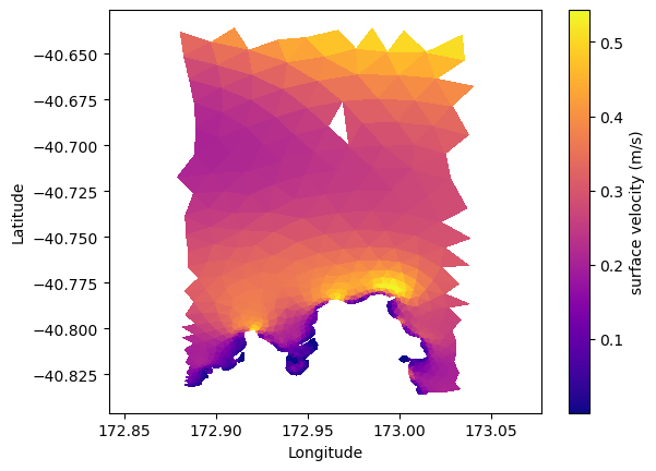
# lets plot the surface, and the depth average horizontal velocity magnitude

# the horizontal velocity variable here is called "hvel"
# ds['hvel'].shape
# (time step, node, depth layer, xy)

# hence to get the surface velocity magnitude (at time step zero)
import numpy as np
hvel_mag_surface = np.linalg.norm(ds['hvel'][0,:,-1,:], axis=1)

plt.tripcolor(lon, lat, triangles, hvel_mag_surface, cmap='plasma')
plt.xlabel('Longitude')
plt.ylabel('Latitude')
plt.axis('equal')
plt.colorbar(label='surface velocity (m/s)')

<matplotlib.colorbar.Colorbar at 0x7f65980f41d0>

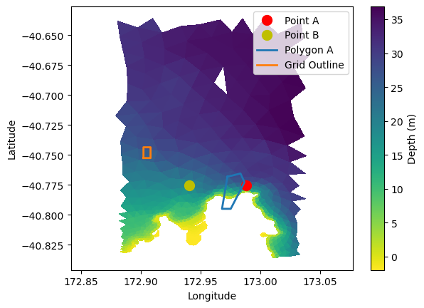
Plotting your release groups

# another thing that we probably want to check that our release locations
# and - if we have some - statistic grids are within the boundary
# so lets take our locations from notebook "C_release_groups.ipynb"

# release_location
# ----------------
point_A = [1599000, 5486200]
point_B = [1595000, 5486200]

polygon_A=[
    [1597682, 5486972],
    [1598604, 5487275],
    [1598886, 5486464],
    [1597917, 5484000],
    [1597300, 5484000],
    [1597682, 5486972],
]

grid_center=[1592000, 5489200]  # location of grid centre
grid_span=[500, 1000]  # size of grid in meters
grid_size=[3, 4]  # rows and columns in grid

# Transform points
point_A_lon, point_A_lat = transformer.transform(point_A[0], point_A[1])
point_B_lon, point_B_lat = transformer.transform(point_B[0], point_B[1])

# Transform polygon
polygon_A_xy = np.array(polygon_A)
polygon_A_lon, polygon_A_lat = transformer.transform(polygon_A_xy[:, 0], polygon_A_xy[:, 1])

# Transform grid outline
grid_center_xy = np.array(grid_center)
grid_span_x, grid_span_y = grid_span

x_min = grid_center_xy[0] - grid_span_x / 2
x_max = grid_center_xy[0] + grid_span_x / 2
y_min = grid_center_xy[1] - grid_span_y / 2
y_max = grid_center_xy[1] + grid_span_y / 2

# Grid outline coordinates (rectangle)
grid_outline_x = [x_min, x_max, x_max, x_min, x_min]
grid_outline_y = [y_min, y_min, y_max, y_max, y_min]
grid_outline_lon, grid_outline_lat = transformer.transform(grid_outline_x, grid_outline_y)

plt.tripcolor(lon, lat, triangles, ds['depth'], shading='flat', cmap='viridis_r')
plt.colorbar(label='Depth (m)')

# Plot overlays
plt.plot(point_A_lon, point_A_lat, 'ro', markersize=10, label='Point A')
plt.plot(point_B_lon, point_B_lat, 'yo', markersize=10, label='Point B')
plt.plot(polygon_A_lon, polygon_A_lat, linewidth=2, label='Polygon A')
plt.plot(grid_outline_lon, grid_outline_lat, linewidth=2, label='Grid Outline')

plt.xlabel('Longitude')
plt.ylabel('Latitude')
plt.axis('equal')
plt.legend()

<matplotlib.legend.Legend at 0x7f65983725d0>