Add your own class#
[This note-book is in oceantracker/tutorials_how_to/]
Here, we will again use the minimal example but this time we add a “user written class”. We try to provide functionally that cover a range of use-cases. However, many scientific applications attempt to illustrate something “new” - i.e. will require a special functionality that we haven’t implemented yet. In those cases, you might want to add this functionality yourself.
We designed OceanTracker in mind and try to make this process easy. In most scenarios you can make use of python “class inheritance” functionality. I.e. you can use one of the already implemented classes e.g. a particle property class and only tweak one ore two methods - typically the “update”-method.
Here we present an example of this. We create new class in a python file in the same directory as your run script. There are other ways to do this that are more robust, but this one is the simplest. The file we will be using here is “my_part_prop.py” and it looks like this
%pycat my_part_prop.py
[38;5;28;01mfrom[39;00m oceantracker.particle_properties._base_particle_properties [38;5;28;01mimport[39;00m (
_BaseParticleProperty,
)
[38;5;66;03m# to avoid accidental parameterization error we use these functions[39;00m
[38;5;66;03m# where we define "valid input" for each configuration variable[39;00m
[38;5;28;01mfrom[39;00m oceantracker.util.parameter_checking [38;5;28;01mimport[39;00m (
ParamValueChecker [38;5;28;01mas[39;00m PVC,
ParameterTimeChecker [38;5;28;01mas[39;00m PTC,
ParameterListChecker [38;5;28;01mas[39;00m PLC,
ParameterCoordsChecker [38;5;28;01mas[39;00m PCC,
)
[38;5;28;01mfrom[39;00m oceantracker.util.numpy_util [38;5;28;01mimport[39;00m possible_dtypes
[38;5;28;01mfrom[39;00m oceantracker.shared_info [38;5;28;01mimport[39;00m (
shared_info [38;5;28;01mas[39;00m si,
) [38;5;66;03m# proces access to all variables , classes and info[39;00m
[38;5;28;01mfrom[39;00m oceantracker.util.numba_util [38;5;28;01mimport[39;00m (
njitOT,
njitOTparallel,
prange,
) [38;5;66;03m# numba decorators to make code fast[39;00m
[38;5;28;01mclass[39;00m TimeAtStatus(_BaseParticleProperty):
[33m"""class to calculate the time each particle spends in a given status"""[39m
[38;5;66;03m# the init method is what is called during the creation of the class instance[39;00m
[38;5;28;01mdef[39;00m __init__(self):
[38;5;66;03m# this calls the parent class method, to maintain its functionality without copying the code[39;00m
super().__init__()
[38;5;66;03m# we add one new default parameter that tells the class which particles to count[39;00m
self.add_default_params(
required_status=PVC(
[33m"moving"[39m, [38;5;66;03m# default type[39;00m
str, [38;5;66;03m# required variable type for this input parameter[39;00m
possible_values=[
key [38;5;28;01mfor[39;00m key, item [38;5;28;01min[39;00m si.particle_status_flags.items() [38;5;28;01mif[39;00m item >= [32m0[39m
],
doc_str=[33m"The particle status to count the time spend"[39m,
),
description=PVC(
[38;5;66;03m# optional description and units are added to part. prop. netcdf variables attributes[39;00m
[33m"total time particle spends in a given status"[39m, [38;5;66;03m# description[39;00m
str,
units=[33m"seconds"[39m,
),
[38;5;66;03m# this will define the data type of the new particle property[39;00m
dtype=PVC([33m"float64"[39m, str, possible_values=possible_dtypes),
)
[38;5;66;03m# during the model setup phase, we run this code[39;00m
[38;5;28;01mdef[39;00m initial_setup(self):
[38;5;66;03m# first we execute the "parent" (_BaseParticleProperty) "initial_setup" method again[39;00m
super().initial_setup()
[38;5;66;03m# next we select, based on user input, the status set for which we will calculate this particle property[39;00m
[38;5;66;03m# this is stored in self.info, where most of the run time properties are stored[39;00m
self.info[[33m"status_value"[39m] = si.particle_status_flags[
self.params[[33m"required_status"[39m]
]
[38;5;66;03m# this will be used to initialize the particle property for each particle during its creation[39;00m
[38;5;66;03m# in our case "0" for zero seconds within the selected status[39;00m
[38;5;28;01mdef[39;00m initial_value_at_birth(self, new_part_IDs):
self.set_values([32m0.0[39m, new_part_IDs)
[38;5;66;03m# the update class is what is called during the "actual" model run.[39;00m
[38;5;66;03m# I.e. after every time step.[39;00m
[38;5;66;03m# Hence, this function will be called the most frequently.[39;00m
[38;5;66;03m# To make it fast, we will create a numba function (_add_time)[39;00m
[38;5;66;03m# Alternatively, you can use numpy function for the "heavy lifting".[39;00m
[38;5;66;03m# Pure python operations tend to be much slower, and might otherwise[39;00m
[38;5;66;03m# slow down your simulation (check the timing information in the caseInfo)[39;00m
[38;5;28;01mdef[39;00m update(self, n_time_step, time_sec, active):
[38;5;66;03m# All we wan't to do here is to accumulate time for each particle in required status[39;00m
[38;5;66;03m# which are currently "active" (e.g. exist, in contrast of those not yet released or removed)[39;00m
[38;5;66;03m# this just contains a dict of all particle properties[39;00m
part_prop = si.class_roles.particle_properties
[38;5;66;03m# add the time (i.e. time step size) that the selected (required status)[39;00m
[38;5;66;03m# particles have been in that state[39;00m
self._add_time(
self.info[[33m"status_value"[39m],
si.settings.time_step,
part_prop[[33m"status"[39m].data,
self.data, [38;5;66;03m# the data of this particle property holds the accumulating time in the required status[39;00m
active,
)
[38;5;28;01mpass[39;00m
[38;5;66;03m# Numba code cannot use classes such as self, as Numba only understands basic python variable types and numpy arrays[39;00m
[38;5;66;03m# the "@njit" decorator - which we slightly tweaked in @njitOTparallel - speeds up the code using numba and uses parallel threads[39;00m
@staticmethod
@njitOTparallel
[38;5;28;01mdef[39;00m _add_time(required_status, time_step, status, total_time, active):
[38;5;66;03m# threaded parallel (prange) for-loop over indices of active particles[39;00m
[38;5;28;01mfor[39;00m nn [38;5;28;01min[39;00m prange(active.size):
n = active[nn]
[38;5;28;01mif[39;00m status[n] == required_status:
total_time[n] += time_step
[38;5;28;01mpass[39;00m
# Notes for debugging if the scripts below fail:
# * These scripts assume that you already installed oceantracker. If you didn't take a look at https://oceantracker.github.io/oceantracker/_build/html/info/installing.html
# * Paths in this directory are relative to the location of the ipython notebook.
#   I.e. On Linux or Mac, running a cell with "!ls" should return a list containing the notebook you are running.

# Checks if the hindcast data is available and downloads them if not
from oceantracker.util.download_data import download_hindcast_data_for_tutorials
download_hindcast_data_for_tutorials()
Hindcast data found locally at ./demo_hindcast
# here we will again use the minimal example (take a look A_minimal_example.ipynb first, if you haven't already)
from oceantracker.main import OceanTracker
import os

ot = OceanTracker()

ot.settings(
    run_output_dir=os.path.join("output", "add_user_written_class"),
    time_step=120.0,  #  2 min time step as seconds
)

ot.add_class(
    "reader",
    input_dir="./demo_hindcast/schsim3D",
    file_mask="demo_hindcast_schisim3D*.nc",
)

ot.add_class(
    "release_groups",
    points=[
        [1595000, 5482600],
        [1599000, 5486200],
    ],
    release_interval=3600,
    pulse_size=10,
)

# here we add "your class"
# you can add it just like any other class
ot.add_class(
    # you describe its type (e.g. particle property)
    "particle_properties",
    # you point it at your class by using its class name (file_name.ClassName)
    class_name="my_part_prop.TimeAtStatus",
    # and you give it a name (just so you know which one is which in case you have multiple version of it)
    # e.g. if you would like to use the TimeAtStatus class to count both the time stranded on the sore, and the time at bottom of the sea
    name="on_bottom_time"
)

case_info_file_name = ot.run()
helper: ----------------------------------------------------------------------
helper: Starting OceanTracker helper class,  version 0.5.2.55
helper:      Python version: 3.11.14 | packaged by conda-forge | (main, Oct 22 2025, 22:46:25) [GCC 14.3.0]
helper: ----------------------------------------------------------------------
helper: OceanTracker version 0.5.2.55  starting setup helper "main.py":
helper: Started
helper: Output is in dir "/home/ls/projects/oceantracker_dev/oceantracker/tutorials_how_to/output/add_user_written_class"
helper:     hint: see for copies of screen output and user supplied parameters, plus all other output
helper:     >>> Note: to help with debugging, parameters as given by user  are in "raw_user_params.json"
helper: >>> Warning: Numba has already been imported, some numba options may not be used (ignore SVML warning)
helper:     hint: Ensure any code using Numba is imported after Oceantracker is run, eg Oceantrackers "load_output_files.py" and "read_ncdf_output_files.py"
helper: ----------------------------------------------------------------------
helper: Numba setup: applied settings, max threads = 32, physical cores = 32
helper:     hint:  cache code = False, fastmath= False
helper: ----------------------------------------------------------------------
helper:       - Built OceanTracker package tree,      0.004 sec
helper:       - Built OceanTracker sort name map,     0.000 sec
helper:   - Done package set up to setup ClassImporter,       0.004 sec
setup: ----------------------------------------------------------------------
setup:  OceanTracker version 0.5.2.55
setup:     Starting user param. runner at 2026-01-22T17:52:30.872429
setup: ----------------------------------------------------------------------
setup:   - Start  field group manager and readers setup
setup:   - Found input dir "./demo_hindcast/schsim3D"
setup:   - Detected reader class_name = "oceantracker.reader.SCHISM_reader.SCHISMreader"
setup:   - Starting grid setup
setup:     - built node to triangles map,     0.000 sec
setup:     - built triangle adjacency matrix,         0.000 sec
setup:     - found boundary triangles,        0.000 sec
setup:     - built domain and island outlines,        0.475 sec
setup:     - calculated triangle areas,       0.000 sec
setup:   - Finished grid setup
setup: --- Hindcast info ----------------------------------------------------
setup:     Hydro-model is "3D", type "SCHISMreader"
setup:         hint: Files found in dir and sub-dirs of "./demo_hindcast/schsim3D"
setup:         Geographic coords = "False"
setup:         Hindcast start: 2017-01-01T00:30:00  end:  2017-01-01T23:30:00
setup:           time step = 0 days 1 hrs 0 min 0 sec, number of time steps= 24
setup:           grid bounding box = [1589789.000 5479437.000] to [1603398.000 5501640.000]
setup:           has:  A_Z profile=True,  bottom stress=False, regrid to sigma=True
setup:           vertical grid type = "LSC", using vertical grid  "Sigma"
setup: ----------------------------------------------------------------------
setup:   - Built barycentric-transform matrix,        0.000 sec
setup:   - Loading reader fields ['tide', 'water_depth', 'water_velocity']
setup:   - Finished field group manager and readers setup,    0.693 sec
setup: ----------------------------------------------------------------------
setup:   - Added 1 release group(s) and found run start and end times,        0.005 sec
setup:   - Starting initial setup of all classes
setup:     - Done initial setup of all classes,       0.003 sec
setup: ----------------------------------------------------------------------
setup:   - Starting "add_user_written_class",  duration: 0 days 23 hrs 0 min 0 sec
setup:       From 2017-01-01T00:30:00 to  2017-01-01T23:30:00
setup:       Time step 120.0 sec
setup:         using: A_Z_profile = False, bottom_stress = False
setup: ----------------------------------------------------------------------
setup:   -  Reading 24 time steps,  for hindcast time steps 00:23 into ring buffer offsets 000:023 ,  for run "None"
setup:       -  read  24 time steps in  0.1 sec, from ./demo_hindcast/schsim3D
setup:   - Starting time stepping: 2017-01-01T00:30:00 to 2017-01-01T23:30:00
setup:     duration  0 days 23 hrs 0 min 0 sec, time step=  0 days 0 hrs 2 min 0 sec
S:   - Opened tracks output and done written first time step in: "tracks_compact_000.nc",     0.006 sec
S: 0000: 00%:H0000b00-01 Day +00 00:00 2017-01-01 00:30:00: Rel:20   : Active:20     Move:20     Bottom:0     Strand:0      Dead:0     Out:   0 Buffer: 4%  step time = 11.1 ms
S: 0030: 04%:H0001b01-02 Day +00 01:00 2017-01-01 01:30:00: Rel:40   : Active:40     Move:40     Bottom:0     Strand:0      Dead:0     Out:   0 Buffer: 8%  step time =  9.1 ms
S: 0060: 09%:H0002b02-03 Day +00 02:00 2017-01-01 02:30:00: Rel:60   : Active:60     Move:60     Bottom:0     Strand:0      Dead:0     Out:   0 Buffer:12%  step time =  5.5 ms
S: 0090: 13%:H0003b03-04 Day +00 03:00 2017-01-01 03:30:00: Rel:70   : Active:70     Move:60     Bottom:0     Strand:10     Dead:0     Out:   0 Buffer:14%  step time =  5.8 ms
S: 0120: 17%:H0004b04-05 Day +00 04:00 2017-01-01 04:30:00: Rel:80   : Active:80     Move:70     Bottom:0     Strand:10     Dead:0     Out:   0 Buffer:16%  step time =  7.0 ms
S: 0150: 22%:H0005b05-06 Day +00 05:00 2017-01-01 05:30:00: Rel:90   : Active:90     Move:80     Bottom:0     Strand:10     Dead:0     Out:   0 Buffer:18%  step time =  8.5 ms
S: 0180: 26%:H0006b06-07 Day +00 06:00 2017-01-01 06:30:00: Rel:100  : Active:100    Move:90     Bottom:0     Strand:10     Dead:0     Out:   0 Buffer:20%  step time = 12.2 ms
S: 0210: 30%:H0007b07-08 Day +00 07:00 2017-01-01 07:30:00: Rel:110  : Active:110    Move:100    Bottom:0     Strand:10     Dead:0     Out:   0 Buffer:22%  step time =  7.2 ms
S: 0240: 35%:H0008b08-09 Day +00 08:00 2017-01-01 08:30:00: Rel:120  : Active:120    Move:110    Bottom:0     Strand:10     Dead:0     Out:   0 Buffer:25%  step time =  5.0 ms
S: 0270: 39%:H0009b09-10 Day +00 09:00 2017-01-01 09:30:00: Rel:140  : Active:140    Move:140    Bottom:0     Strand:0      Dead:0     Out:   0 Buffer:29%  step time =  7.9 ms
S: 0300: 43%:H0010b10-11 Day +00 10:00 2017-01-01 10:30:00: Rel:160  : Active:160    Move:160    Bottom:0     Strand:0      Dead:0     Out:   0 Buffer:33%  step time =  8.9 ms
S: 0330: 48%:H0011b11-12 Day +00 11:00 2017-01-01 11:30:00: Rel:180  : Active:180    Move:180    Bottom:0     Strand:0      Dead:0     Out:   0 Buffer:37%  step time = 10.6 ms
S: 0360: 52%:H0012b12-13 Day +00 12:00 2017-01-01 12:30:00: Rel:200  : Active:200    Move:200    Bottom:0     Strand:0      Dead:0     Out:   0 Buffer:41%  step time =  8.8 ms
S: 0390: 57%:H0013b13-14 Day +00 13:00 2017-01-01 13:30:00: Rel:220  : Active:220    Move:205    Bottom:0     Strand:15     Dead:0     Out:   0 Buffer:45%  step time =  7.1 ms
S: 0420: 61%:H0014b14-15 Day +00 14:00 2017-01-01 14:30:00: Rel:240  : Active:240    Move:221    Bottom:0     Strand:19     Dead:0     Out:   0 Buffer:50%  step time =  8.2 ms
S: 0450: 65%:H0015b15-16 Day +00 15:00 2017-01-01 15:30:00: Rel:250  : Active:250    Move:193    Bottom:0     Strand:57     Dead:0     Out:   0 Buffer:52%  step time = 12.6 ms
S: 0480: 70%:H0016b16-17 Day +00 16:00 2017-01-01 16:30:00: Rel:260  : Active:260    Move:199    Bottom:0     Strand:61     Dead:0     Out:   0 Buffer:54%  step time =  7.7 ms
S: 0510: 74%:H0017b17-18 Day +00 17:00 2017-01-01 17:30:00: Rel:270  : Active:270    Move:198    Bottom:0     Strand:72     Dead:0     Out:   0 Buffer:56%  step time =  9.9 ms
S: 0540: 78%:H0018b18-19 Day +00 18:00 2017-01-01 18:30:00: Rel:280  : Active:280    Move:208    Bottom:0     Strand:72     Dead:0     Out:   0 Buffer:58%  step time =  8.7 ms
S: 0570: 83%:H0019b19-20 Day +00 19:00 2017-01-01 19:30:00: Rel:290  : Active:290    Move:222    Bottom:0     Strand:68     Dead:0     Out:   0 Buffer:60%  step time =  7.7 ms
S: 0600: 87%:H0020b20-21 Day +00 20:00 2017-01-01 20:30:00: Rel:300  : Active:300    Move:236    Bottom:0     Strand:64     Dead:0     Out:   0 Buffer:62%  step time =  7.3 ms
S: 0630: 91%:H0021b21-22 Day +00 21:00 2017-01-01 21:30:00: Rel:320  : Active:320    Move:301    Bottom:0     Strand:19     Dead:0     Out:   0 Buffer:66%  step time =  7.6 ms
S: 0660: 96%:H0022b22-23 Day +00 22:00 2017-01-01 22:30:00: Rel:340  : Active:340    Move:325    Bottom:0     Strand:15     Dead:0     Out:   0 Buffer:70%  step time =  7.8 ms
S: 0690: 100%:H0022b22-23 Day +00 23:00 2017-01-01 23:30:00: Rel:360  : Active:360    Move:360    Bottom:0     Strand:0      Dead:0     Out:   0 Buffer:75%  step time = 14.8 ms
S: --- Closing all classes ----------------------------------------------
S: Converting compact track files to rectangular format (to disable set reader param convert=False)
S:     hint: reading from dir /home/ls/projects/oceantracker_dev/oceantracker/tutorials_how_to/output/add_user_written_class
S:     - Finished "tracks_rectangular_000.nc",        0.117 sec
S:     - Conversion complete,         0.117 sec
S: Removing compact track files output after conversion
end: ----------------------------------------------------------------------
end: Finished "add_user_written_class"
end:     Timings: total =   8.6 sec
end:         Setup                          1.17 s   13.6%
end:         Find initial horizontal cell   1.43 s   16.5%
end:         Reading hindcast               1.19 s   13.8%
end:         Find horizontal cell           2.93 s   33.9%
end:         Find vertical cell             1.85 s   21.4%
end:         Interpolate fields             2.29 s   26.5%
end:         Update custom particle prop.   0.01 s    0.1%
end:         Update statistics              0.00 s    0.0%
end:         Update event loggers           0.00 s    0.0%
end:         RK integration                 0.62 s    7.2%
end:         Releasing particles            0.10 s    1.2%
end:         Close down                     8.87 s   102.7%
end:         resuspension                   0.01 s    0.1%
end:         dispersion                     0.05 s    0.6%
end:         tracks_writer                  0.08 s    0.9%
end: ----------------------------------------------------------------------
end: Finished "add_user_written_class",  started: 2026-01-22 17:52:30.864069, ended: 2026-01-22 17:52:39.501602
end:       Computational time = 0:00:08.637548
end:       Max. memory used 112.31 GB
end: --- Issues    (check above,  any errors repeated below) --------------
end:     0 errors,    0 strong warnings,   1 warnings,   1 notes
end: --- Successful completion: output in "output/add_user_written_class" -
# you will find its output here
print(case_info_file_name)
/home/ls/projects/oceantracker_dev/oceantracker/tutorials_how_to/output/add_user_written_class/caseInfo.json
Read and plot output#
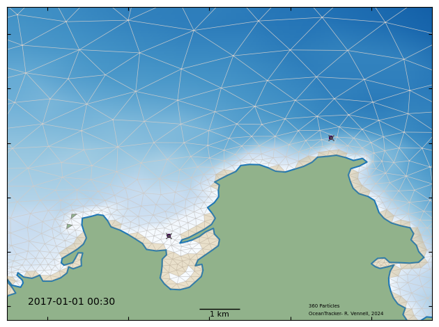
To take a quick look we can visualize the the particle properties in an animation. We can pass the particle property (“on_bottom_time”) to the animtion function color_using_data variable. The color will then represent the amount of time that this particle has spend on the bottom.
from oceantracker.read_output.python import load_output_files
from oceantracker.plot_output import plot_tracks
from IPython.display import HTML


tracks = load_output_files.load_track_data(case_info_file_name)
anim = plot_tracks.animate_particles(
    tracks,
    axis_lims=[1591000, 1601500, 5479500, 5491000],
    colour_using_data=tracks["on_bottom_time"],
    back_ground_depth=True,
    show_grid=True,
    show_dry_cells=True,
    interval=50,
)
# HTML(anim.to_html5_video())  # this is slow to build!
Merging rectangular track files
     Reading rectangular track file "tracks_rectangular_000.nc"
animate_particles: color map limits None None